Written by: Tim Rudderow, CEO | Mount Lucas Management
Over the years we all have learned about return and standard deviation, the first and second “moments” of asset class return distributions. But there are more moments to every distribution and the third, skew, is important to understand as you consider your asset allocation model. Put simply, skew tells you which way the big moves in the return series lean. We all know the stock market goes up on the escalator and down on the elevator – up gradually, down fast. That means the return distribution has negative skew. In the article below, we will go through the details of an asset with positive skew, Managed Futures. We will show how positive skew can impact portfolio returns, and how strategy decisions by your manager may be impacting that skew.
Sharpe or Skew?
Managed Futures offers this promise – uncorrelated returns with the potential for crisis protection. How an allocator chooses to allocate to this asset class is important. Do they judge managers by best risk-adjusted performance? Or do they judge managers by how they improve the risk-adjusted performance of the total portfolio? Do they view the asset as an absolute return element, prioritizing Sharpe Ratio, or as a portfolio element prioritizing diversification? Assuming the latter, prioritizing the addition of positive skew is critical to crisis diversification, offsetting the historically negative skew of the equity market and creating a better total portfolio.
Typical Managed Futures managers employ a risk-controlled approach called volatility, or “vol”, targeting. In essence, vol targeting involves increasing exposure when volatility is low and reducing it when volatility is high. Historically this has improved manager Sharpe ratio at the expense of skew.
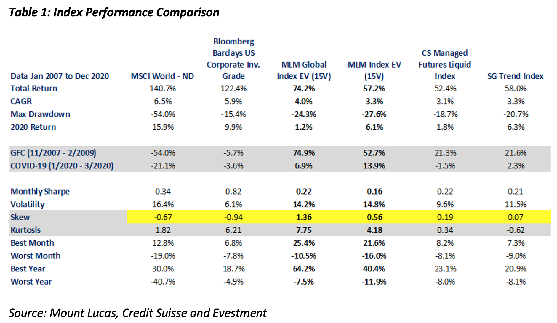
In Table 1 we compare the MLM Index EV and MLM Global Index EV to the SG Trend Index (index of manager returns) and the Credit Suisse (CS) Managed Futures Liquid Index (vol-adjusted price-based index) and show skew and correlation statistics. The MLM Index EV and MLM Global Index EV, price-based benchmarks of Managed Futures, are constructed a bit differently. While implementing similar trend following algorithms, positions are sized on exposure, not vol. Notice the skew line, highlighted in yellow. Stocks and credit show negative skew, while Managed Futures are positive. This makes intuitive sense; trend following tends to crash up while equity markets tend to crash down. However, the vol adjusted Managed Futures indices have a much lower positive skew.
Let’s see how the skew differences impact portfolio outcomes.
You Shouldn’t Bring a Knife to a Gunfight!
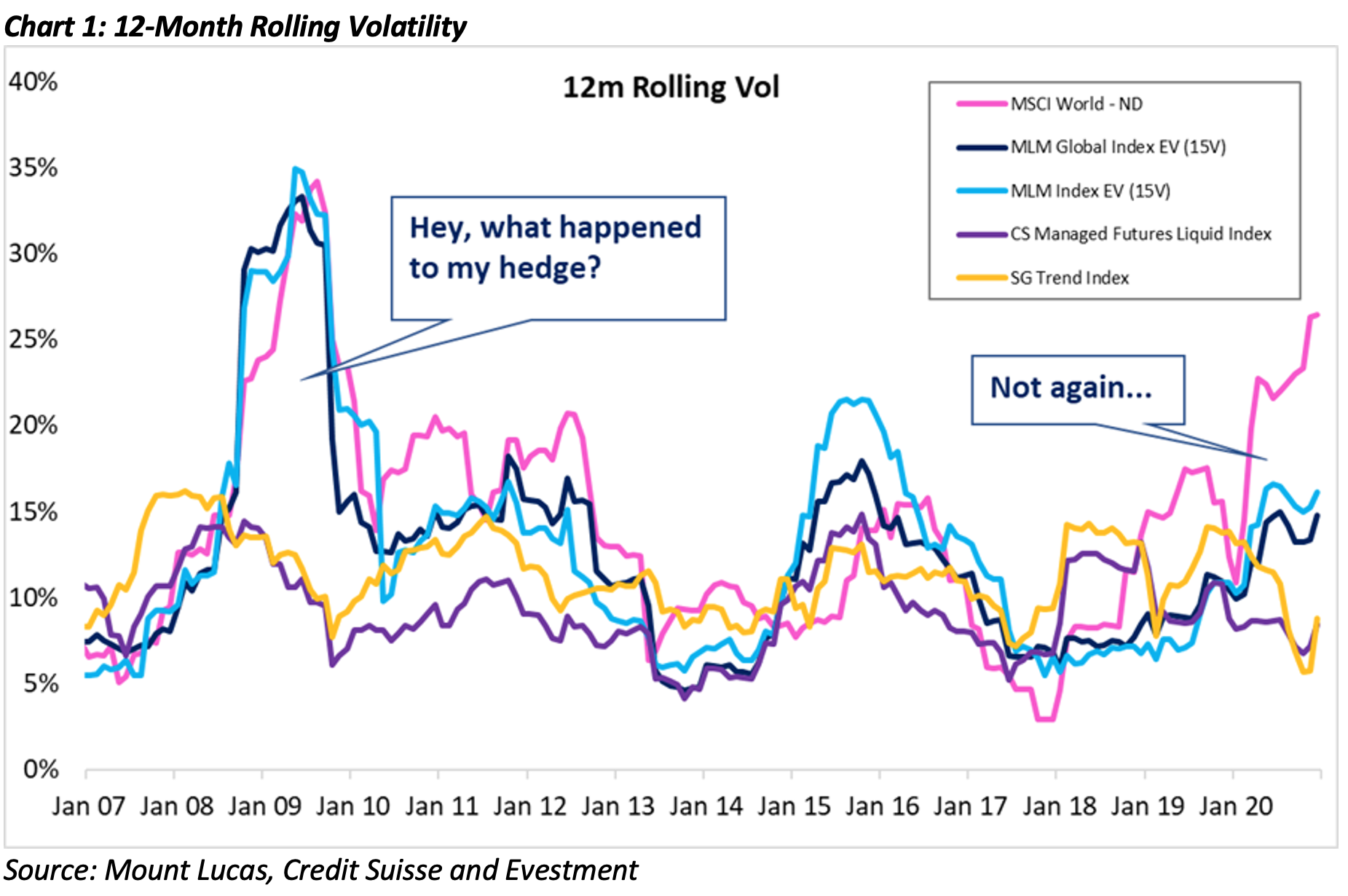
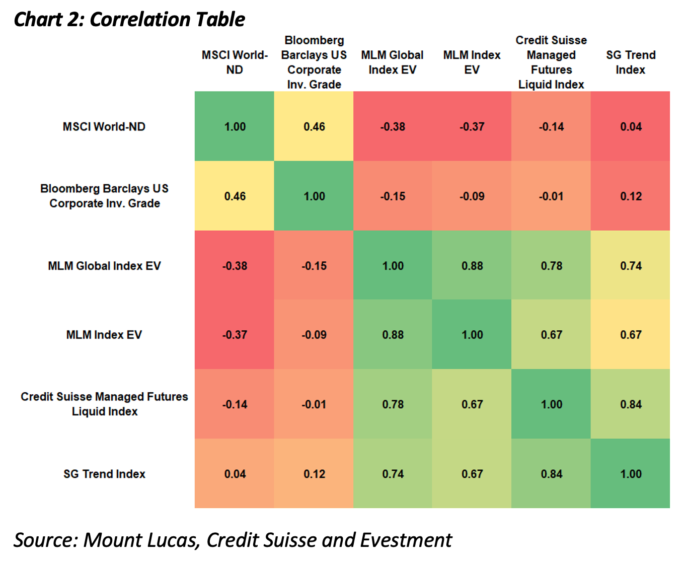
Stocks and credits are negatively skewed and historically have had large drawdowns. Neither asset class is volatility adjusted. If you are optimizing for the whole, and are rebalancing, you ideally need diversifying assets that have a negative or low correlation and positive skew. The next chart is a comparison of rolling 12-month volatility for all the indices in Table 1. Notice that the volatility of the MLM Indices matches the volatility of stocks and credit, whereas the other Managed Futures indices control volatility. That’s good for Sharpe, but bad for the portfolio. Correlations in Chart 2 bear this out, with higher negative correlation between the MLM Indices and stocks and credit.
Practical Examples
Cast your mind back to late 2008 into 2009 when things were really going wrong. Stocks were plummeting, credit markets were freezing. At the same time, the USD was going up, crude oil was dropping precipitously, and the US Treasury market was rallying. See the impact at the position level of a representative model that vol adjusts vs one that does not, using the Nasdaq as the example.
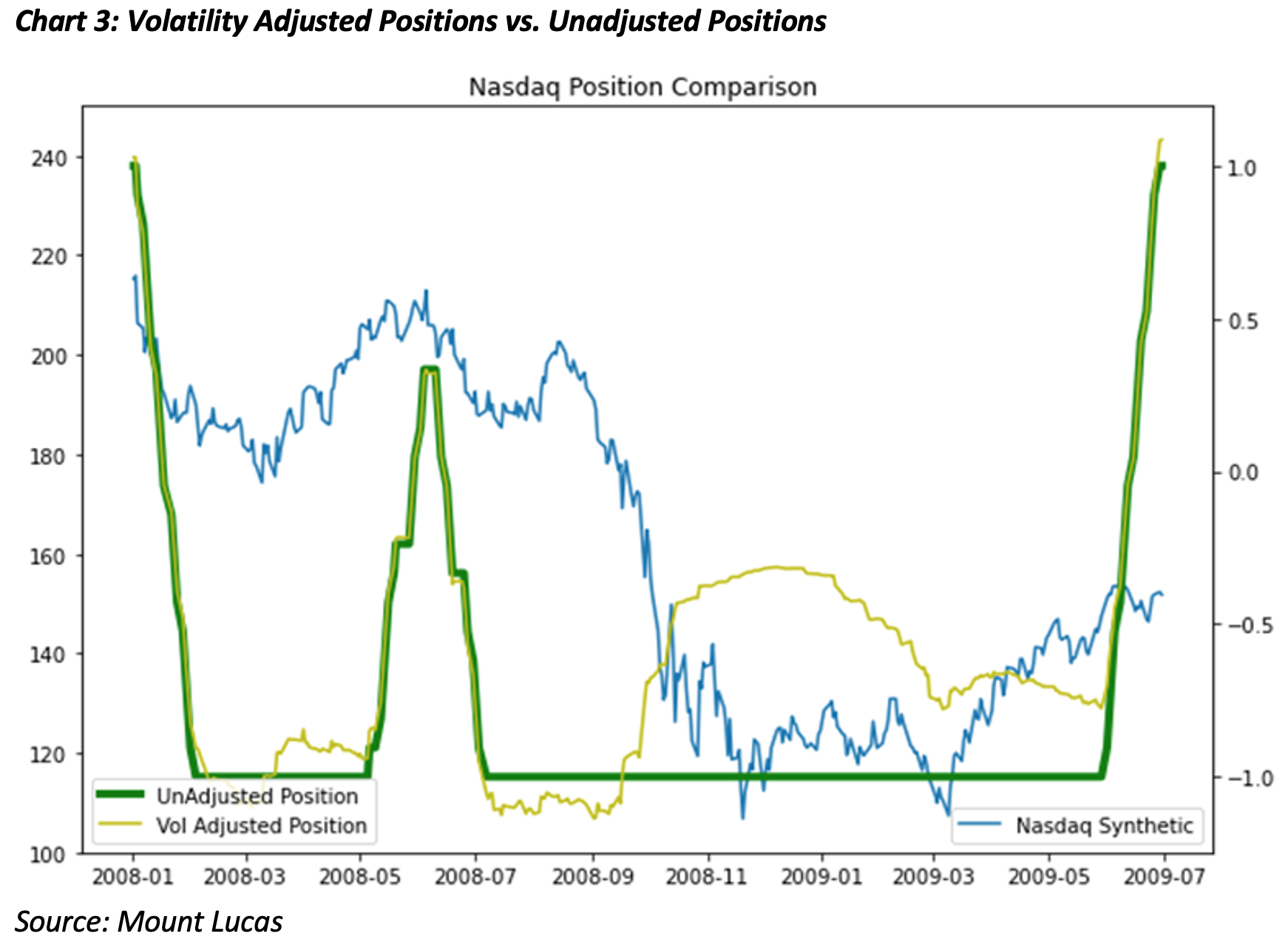
Volatility adjusting positions reduces the diversification benefit at the worst time. The Nasdaq began to fall, the trend following component of the models moved short. The volatility adjustment process reduces the short as realized volatility picks up on the down move around the Lehman collapse. In this representative example, the short is reduced by some 60%.
In the next chart we compare the volatility adjusted model to the unadjusted model, you can see the unadjusted volatility approach has higher returns when you need them most. When using this approach, it is critically important that that portfolio elements are rebalanced. Even though returns in this example end up in about the same spot, at the portfolio level the sequence matters. The extra gains are monetized, the Managed Futures allocation is sold down, and more stock is bought at lower levels.
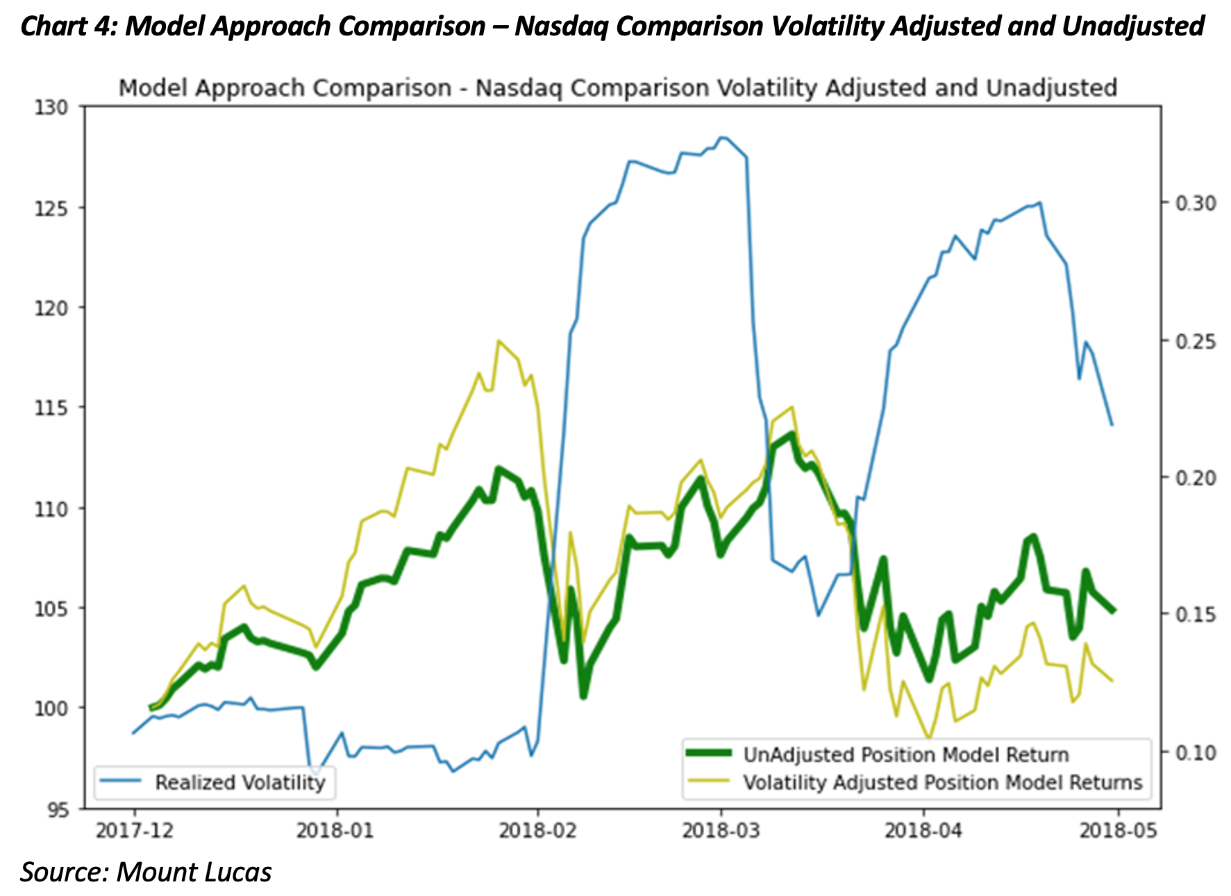
Volatility adjusting can also be detrimental, given that equity prices and vol are negatively correlated. In early 2018, volatility collapsed until it didn’t. As volatility adjusting models increased position sizes in response to falling realized volatility, they are making the case that risk is falling, which is dangerous in our view. When the market fell and fell quickly, they took larger losses as they were at max positions. In a portfolio context this reduces the portfolio diversification benefit to the investor, particularly when this is applied to equity index markets.
A Better Portfolio
When modeling a portfolio with stocks and credits, the different approach is clear. In the example below, we start with a portfolio that holds 50% each stocks and credit. Then we add some vol-adjusted Managed Futures and some leverage to create a portfolio with 40% stocks, 40% credit, and 60% in CS Liquid Managed Futures. For the last two portfolios, we swap in the MLM Global Index EV and the MLM Index EV at the same 60% allocation for Managed Futures.
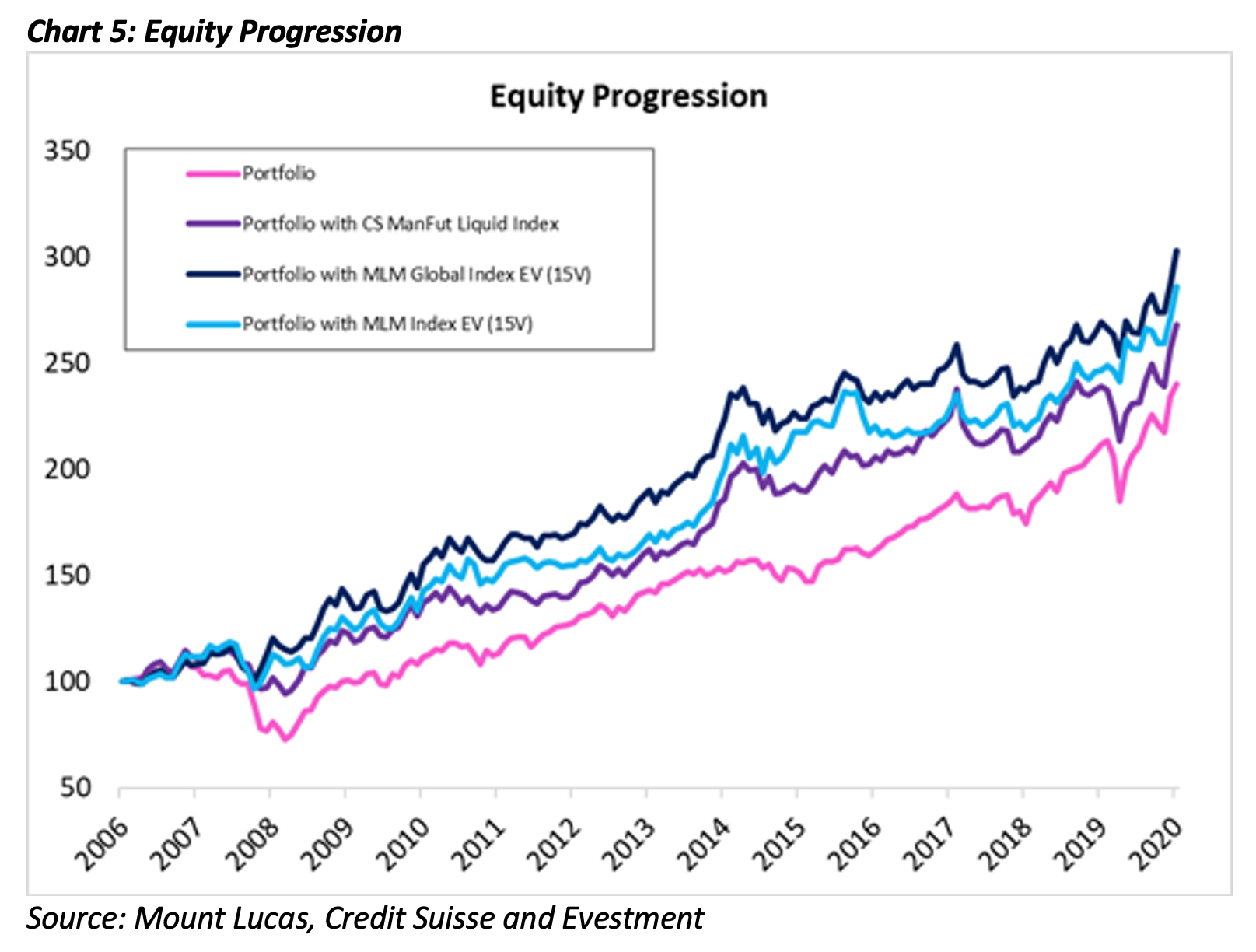
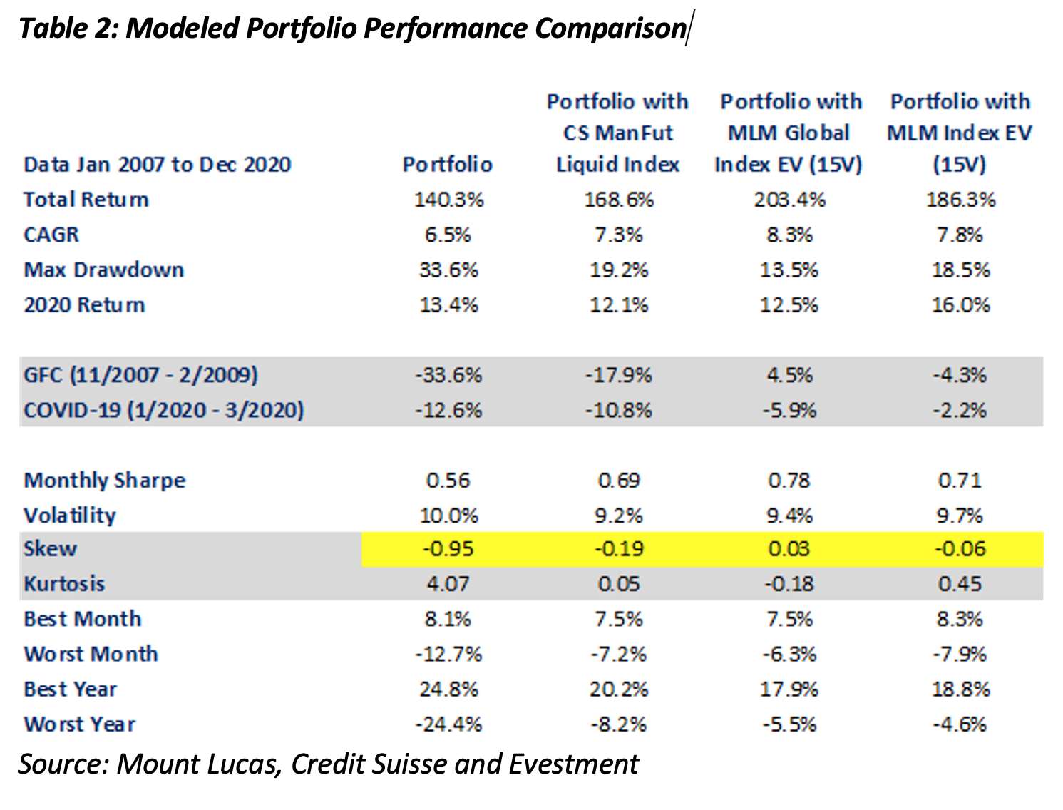
Note the skew changes at the portfolio level – typical portfolios are negatively skewed and adding an uncorrelated positively skewed strategy takes the overall portfolio to zero skew. Drawdowns are much reduced, portfolio Sharpe ratio increases, overall portfolio volatility goes down.
Conclusion
The Covid crisis (Jan 2020 to Mar 2020) provides a complete example in a compact period. Typical trend managers were very long equity December through February, as volatility was still quite low. When markets broke, volatility increased, and the exposure of the trend shorts was proportionately reduced. The same was true in other markets like energy. The MLM Index approach, using constant exposure and thus increased skew, provided better returns over this difficult period. If its diversification you want, ignore the siren song of Sharpe, and go for the skew.


